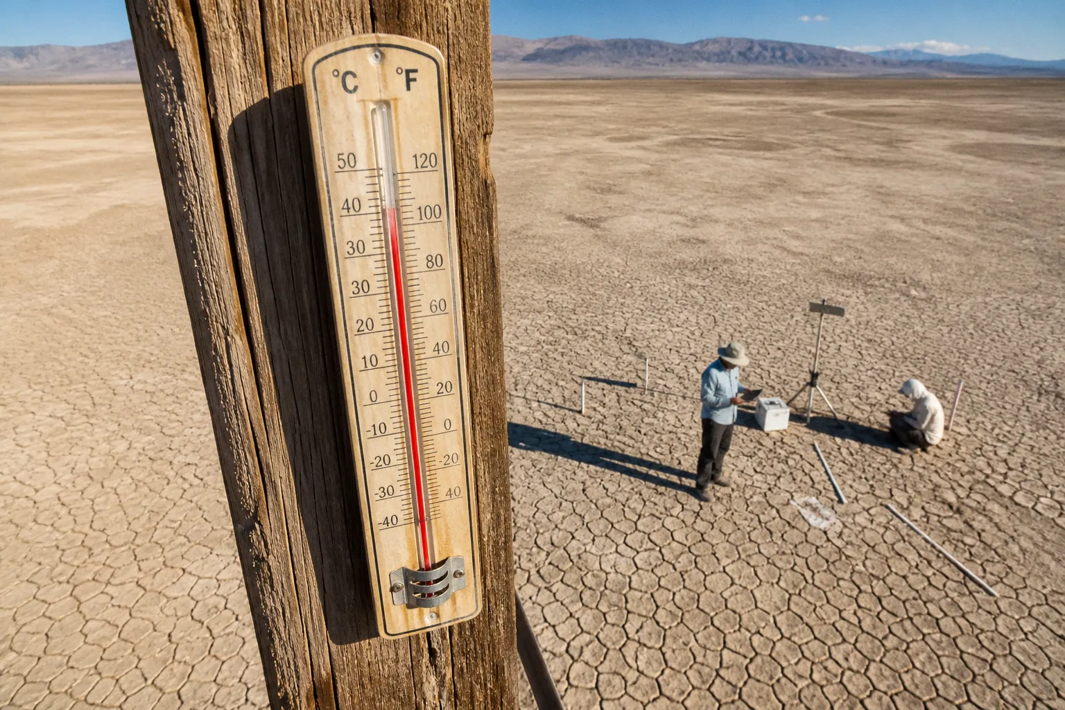
That question sits at the centre of the CMIP6 climate models high sensitivity debate. Some CMIP6 models respond much more strongly to a doubling of atmospheric carbon dioxide than earlier models did, with a small but significant group producing warming levels that appear difficult to reconcile with the temperature record. Yet it would be a mistake to treat the entire modelling effort as one faulty instrument. The real story is more useful than that: climate scientists have been learning how to distinguish a broad ensemble of possibilities from the subset that best fits what the Earth has already shown us.
Compare car rental deals in United Kingdom
See available offersPartner link — DiscoverCars comparisonTo understand why this matters, we need to follow the model output through its own lifecycle — from the underlying physics, to the historical record, to the projections used in policy and regional planning.
From CMIP5 to CMIP6: a wider sensitivity range
Climate models are not crystal balls. They are large numerical systems that represent the atmosphere, ocean, ice, land, clouds and carbon cycle, then calculate how those components interact as conditions change. The Coupled Model Intercomparison Project, or CMIP, gives research groups around the world a shared framework for running and comparing those models.
CMIP5 supported the climate projections used around the time of the IPCC Fifth Assessment Report, published in 2013. Its models placed equilibrium climate sensitivity — usually shortened to ECS — between 2.1°C and 4.7°C, with a mean of 3.3°C.
ECS is a deliberately slow and idealised measure. It asks how much the global average surface temperature would eventually rise after atmospheric carbon dioxide doubles, once the climate system has had time to reach a new equilibrium. The real world does not wait patiently for equilibrium: emissions continue, oceans absorb heat, ice sheets respond over long periods, and atmospheric circulation keeps moving energy around. Still, ECS is a valuable way to compare the basic strength of the climate system’s response.
CMIP6, the next generation, expanded that range considerably. Its models produced ECS values from 1.8°C to 5.6°C, with a mean of 3.9°C. More than a quarter of the CMIP6 models have sensitivities above 4.7°C, and roughly a fifth simulate at least 5°C of warming following a doubling of carbon dioxide.
At first glance, the higher mean can look like a simple revision upwards: perhaps the old models were too conservative and the new ones have corrected the record. But the increase did not come evenly from every part of the model system. Much of it came from a particular change in how some models represented low clouds, especially in the Southern Hemisphere outside the tropics.
That distinction is important. A model can be more sophisticated in one area and still produce an exaggerated response if a newly represented feedback is too strong. More detail does not automatically mean more realism. Sometimes adding another thread to the fabric reveals a stronger pattern; sometimes it exposes where the stitching still needs work.
A wider model range is not the same as a wider range of equally credible futures.
The IPCC’s assessed likely range for ECS in its Sixth Assessment Report was 2.5°C to 4.0°C. That range did not simply copy the lowest and highest values produced by CMIP6. Instead, the assessment combined model results with observations and several independent lines of evidence.
This is the first key to the debate over whether CMIP6 models are too hot: the headline range of an ensemble is not the final scientific judgement. Models are evidence, but they are not counted as votes in a contest where every member gets equal weight.
The cloud problem beneath the headline
Why do clouds matter so much? Because they sit at the point where sunlight enters the climate system and infrared heat leaves it. A layer of low cloud can reflect incoming shortwave sunlight back into space, cooling the surface. If that cloud cover becomes thinner, less reflective or less extensive as the planet warms, more sunlight reaches the surface. The initial warming then receives an additional push.
This is a climate feedback. The original change — in this case, the warming caused by increased greenhouse gases — alters another part of the system, which either reinforces or reduces the initial change.
In the CMIP6 models with especially high ECS, the most important difference from CMIP5 was an enhanced shortwave low-cloud feedback. The effect is concentrated mainly in the Southern extratropics, poleward of 30° south. In plain terms, these models respond to warming by reducing the cooling influence of certain low clouds more strongly than earlier models did.
That sounds like a narrow technical detail, but it is precisely the kind of detail that can alter the global projection. Clouds are not painted onto a fixed map. They form and dissolve according to temperature, humidity, atmospheric circulation, turbulence and the properties of the surface below. Their behaviour is also difficult to observe consistently over long periods, which makes it hard to test every part of the feedback directly.
The result is not that scientists know nothing about clouds. Rather, clouds remain one of the hardest pieces of the climate system to reclaim from uncertainty and place into a stable, tested loop of observation and prediction.
Some high-sensitivity models reproduce the observed cloud behaviour reasonably well in particular regions or situations. Others show a response that appears too strong when compared with historical observations. The disagreement is therefore not a simple choice between cloud feedback being real or imaginary. The question is how large the feedback is, where it operates, and whether a model’s cloud response remains credible when the model is asked to reproduce the climate of the recent past.
What the historical record tells us
A climate model is not judged only by the future it projects. Before we use it to explore the end of this century, we can ask it to reproduce the climate that has already happened.
This test is not as straightforward as placing a thermometer next to a computer and marking the model right or wrong. Models simulate broad patterns and averages, while observations are unevenly distributed across land and ocean. Volcanic eruptions, solar changes, industrial aerosols and natural variability also affect the observed record. A model may miss the precise timing of a short-lived event without being useless for long-term climate analysis.
Even so, persistent errors matter.
Many of the CMIP6 models with the highest sensitivities struggle to reproduce the pattern of twentieth-century warming accurately. Some simulate relatively little warming across much of the twentieth century, followed by a steep warming spike in recent decades that is more pronounced than the observed record. Their long-term response may be physically possible in the abstract, but their path through the climate history we know can look implausible.
This is where climate modelling projections accuracy becomes a practical question rather than a contest over which number sounds most alarming. If a model cannot reproduce important features of the historical record, we should be cautious about treating its far-future output as an equal partner in an average.
There is another complication: a model can be too cool in one period and too warm in another while still landing near the observed average over a longer interval. A single score can hide the shape of the error. Climate scientists therefore look at several behaviours at once:
- How the model represents the twentieth-century temperature trend.
- Whether it captures the response to major volcanic eruptions.
- How it handles the warming of the oceans, not just the air above land.
- Whether its regional patterns of warming and precipitation resemble observations.
- Whether the feedbacks responsible for its sensitivity are consistent with physical evidence.
A model’s history is not a perfect preview of its future, but it is a form of quality control. We would not use a reclaimed material in a new product without checking how it behaved under stress. Climate models deserve the same practical scrutiny.
Why the recent warming spike matters
The recent decades contain a particularly useful test because greenhouse gas concentrations have risen substantially and global temperatures have also climbed. A model that responds too weakly early on and then too sharply later may be revealing a problem in how its feedbacks interact.
In high-sensitivity CMIP6 models, the combination of a strong cloud feedback and other model characteristics can produce an unusually steep recent warming trajectory. That does not mean the observed warming is false, nor does it mean every model with a high ECS is automatically disqualified. It means the output needs to be constrained by the full body of evidence rather than accepted because it belongs to the newest modelling generation.
This distinction protects us from two equally unhelpful reactions. One is to dismiss all CMIP6 models as overheated. The other is to assume that the latest and most complex model must be right simply because it is latest and most complex.
Why the IPCC did not use a raw CMIP6 average
The phrase “model average” can suggest something more neutral than it really is. Imagine an ensemble in which every model contributes one result, regardless of whether it reproduces observed warming, cloud behaviour or ocean heat uptake well. The arithmetic mean may be easy to calculate, but it does not necessarily represent the most likely future.
The IPCC Sixth Assessment Report, published in 2021, did not rely on a direct, unweighted average of raw CMIP6 projections for its headline warming assessments. Instead, it used observational constraints and multiple lines of evidence to assess which parts of the model range were more credible.
That approach is sometimes described as weighting or filtering the ensemble, but the underlying idea is simple: models should be evaluated against the physical world. If a model’s sensitivity is very high and its historical behaviour is also inconsistent with observations, that combination should affect how much confidence we place in its long-term projection.
The assessment process did not erase high-sensitivity possibilities. Nor did it declare that they could never occur. Rather, it placed them within a broader probability judgement. A low-probability, high-impact outcome can remain important for risk planning even when it is not treated as the central estimate.
This is one reason the question are CMIP6 models too hot cannot be answered with a single yes or no. Some are likely too sensitive for use as equal-weight members of a simple average. The CMIP6 framework as a whole, however, remains valuable because it contains a range of model behaviours and allows researchers to investigate why they differ.
The shift from raw averages to constrained projections is also a reminder that climate science is not only about running larger simulations. It is about deciding how model information should be used. The work happens before the number reaches a policy document, a coastal plan or an infrastructure budget.
What changes at the regional scale
Global averages are useful for describing the overall direction of climate change, but decisions are made in particular places. A water manager needs to know about river flows. A city needs to plan for heat. A road authority needs to understand freeze-thaw cycles, heavy rainfall and permafrost stability. Regional projections therefore need more than a global temperature number copied into a local report.
Studies focused on Canada illustrate how much the choice of models can matter. Under high-emissions scenarios, applying observational constraints to reduce the influence of the hottest models has produced end-of-century temperature projections that are 2°C to 3°C cooler than unconstrained ensemble averages in some regional analyses.
That is not a trivial adjustment. A difference of several degrees can change estimates of wildfire conditions, crop suitability, snowpack duration, cooling demand and the timing of infrastructure failure. It can also affect how a government compares adaptation options. A bridge, reservoir or building designed for one range of future conditions may perform very differently under another.
But cooler constrained projections should not be misread as reassurance that climate risks are modest. A projection can be lower than an unconstrained average and still represent severe warming, especially under high emissions. The point of the constraint is not to make the future look comfortable. It is to make the range more physically defensible.
A more useful way to compare model outputs
When we compare CMIP6 projections, the most useful questions are not simply which model gives the highest number. We should ask:
- Does the model reproduce the observed temperature history without relying on an implausible combination of compensating errors?
- Is its high sensitivity driven by a feedback supported by observations and independent physical understanding?
- Does it behave credibly across both global and regional patterns?
- Are we looking at a raw ensemble average or an assessment that has been constrained by observations?
- Is the projection being used to estimate a central expectation, or to explore a high-impact possibility?
Those questions make room for uncertainty without turning uncertainty into fog. They also help us separate three different things that are often bundled together: the range of model output, the assessed likelihood of each part of that range, and the consequences of preparing for a particular outcome.
A planning authority may reasonably examine a high-warming case even if it is not the central estimate. A scientific assessment may reasonably give greater weight to models that reproduce the historical record. Both actions can be sensible at the same time.
The useful question is not whether a model is frightening enough. It is whether its behaviour earns our confidence.
What the high-sensitivity debate does — and does not — tell us
The debate has sometimes been presented as evidence that climate projections are either collapsing or becoming dramatically worse. Neither interpretation is sound.
The high-sensitivity CMIP6 models have exposed a real challenge in climate modelling: changes in the representation of low clouds can produce a much stronger overall response to carbon dioxide. They have also shown why model development needs to be paired with careful evaluation against observations.
At the same time, the existence of hot models does not disprove climate change, make warming harmless or invalidate the wider evidence for human-caused warming. It also does not mean all CMIP6 models are systematically flawed. The problem concerns a subset of models with exceptionally high ECS and, in many cases, a less convincing account of historical temperature change.
Nor does a lower constrained estimate remove the need for urgent emissions reductions. The difference between a central projection and a high-end projection may influence the scale of adaptation required, but it does not reverse the direction of risk. Every additional increment of warming affects heat extremes, ice loss, ecosystems, oceans and the likelihood of compound hazards.
The practical lesson is to stop treating model ensembles as a single undifferentiated pile of numbers. We need to know what each projection contains, what evidence supports it and where its weaknesses lie.
That is a more mature relationship with uncertainty. We do not need to discard the model because one component is imperfect. We need to understand which parts of its output can be used confidently, which require adjustment and which are best kept as stress tests for difficult decisions.
A better loop between models and observations
The CMIP6 debate is ultimately a story about feedback — not only the physical feedbacks inside the climate system, but also the feedback loop between models and the world they are designed to describe.
Observations reveal where a model’s assumptions hold and where they begin to fray. Those findings guide the next generation of model development. New models produce more detailed projections, which are then tested again against temperatures, clouds, ocean heat, ice and rainfall. The loop is not a sign of failure. It is how scientific tools become more useful.
For readers, the clearest takeaway is this: when you encounter a dramatic climate projection, look for the path it took before arriving on the page. Was it drawn from a raw average? Was it constrained by observations? Is it describing a central estimate or a high-impact scenario? Which physical feedback is driving the result?
Those details may sound technical, but they change the meaning of the number.
CMIP6 has not delivered one final answer about the planet’s equilibrium climate sensitivity. It has made the spread of possible answers more visible, while also revealing that some of the hottest results need to be treated with caution. The IPCC AR6 response — weighing model output against the observed climate and other evidence — is therefore not a retreat from modelling. It is a way of reclaiming the useful signal from an ensemble that contains both strong tools and overstated responses.
The future will not arrive as a model average. It will arrive through the atmosphere, oceans, streets, farms and coastlines we share. Our job is to use the models honestly: neither smoothing away the high-end risks nor allowing the hottest projections to stand in for the whole climate system.